
Top 30 Powerful Excel Formulas Every Business Analyst Should Know!
Whether you’re dealing with financial reports, sales trends, or organising a project, these formulas turn chaotic data into meaningful information. These formulas range from basic ones like SUM and AVERAGE to more sophisticated ones like VLOOKUP and INDEX-MATCH. But the work does not stop at mere calculation.
It goes beyond this; it helps you to make better decisions within a short period. So, if you are keen to learn about all those complicated Excel formulas, this blog will help you get hands-on with them as business analysts and see how they are essential in data analysis. So, why wait? Let’s take this journey with you and convert those scary numbers into actionable insights!
Table Of Content
Top 30 Excel Formulas And Functions
Pro Tips for Mastering Microsoft Excel
In the End
Frequently Asked Questions
Top 30 Excel Formulas And Functions
Most Excel formulas for business analysts are common, but did you know they don’t work by hearing? Try this kind of formula instead, which can be used in software as simple and user-friendly as Excel to help simplify a complex set of data:
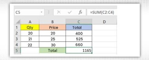
1. SUM
The function SUM(), as its name implies, sums up the addition operation by adding together a range of selected cell values. If you want to find the total sales for several different units, just enter the formula =SUM(C2:C4).
By doing this, it will automatically sum up 400, 525 and 660 to give 1585 in cell C5. Excel is a great tool when it comes to data management skills, and if you want to broaden your skills, it’s valuable to learn how to import data into R from Excel, CSV, text, and XML.
*janbasktraining.com
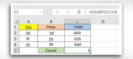
2. COUNT
The COUNT function in Excel is shown as =COUNT(Start Cell: End Cell) in its list of functions. This function counts cells with numbers only. It does not count blank cells and non-numeric format cells.
When counting the range from C1 to C4, it counts four cells normally, but the COUNT function counts only three of them because they have the numeric data, while it skips the cell with the label “Total.” If you want to count all cells with numeric values, text, or other formats, use the COUNTA() function. This method also does not count blank cells.
*janbasktraining.com
3. INDEX MATCH
The INDEX MATCH combination serves as an excellent alternative to the more traditional VLOOKUP or HLOOKUP functions, which have certain limitations. This powerful duo consists of two distinct functions:
- INDEX: This function retrieves the value of a cell based on specified row and column numbers within a table.
- MATCH: This function identifies the position of a cell within a given row or column.
4. AVERAGE
The AVERAGE() function focuses on calculating the mean of a specified range of cell values. To find the average of selected cells, one would input the formula =AVERAGE(Cell 1, Cell 2, Cell 4). Excel will automatically compute the average and allow the user to store the result in a cell of their choosing.
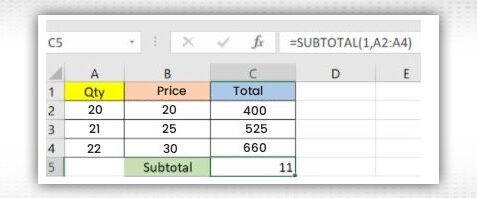
5. SUBTOTAL
*janbasktraining.com
The SUBTOTAL() function is particularly useful for returning a subtotal in a database. For example, if you want to calculate a subtotal for the range A2 to A4, you would use the formula =SUBTOTAL(1, A2:A4). In this context, the number “1” signifies that you are calculating the average. Thus, the function will compute the average of the specified range, resulting in a value of 11, which can be stored in cell C5.
Excel formulas for business analysts are widely utilised in both public and private sectors, especially for careers in data analytics. For those interested in this field, exploring a detailed guide on the data analytics career path can provide deeper insights and understanding.
6. DATE
The DATE Excel formula for business analysts is structured as =DATE(year, month, day). This powerful formula generates a date based on the values entered within the parentheses, which can also include references to other cells. For instance, if cell A1 contains the year 1999, B1 holds the month 9 (September), and C1 has the day 1, entering =DATE(A1, B1, C1) will return the date 9/1/1999. This function is particularly useful for creating dates dynamically based on changing data, which enhances the flexibility of your spreadsheets.

7. ARRAY
The array function in Excel allows you to perform operations on multiple values simultaneously, using the format {=(Start Value 1:End Value 1)*(Start Value 2:End Value 2)}.
By pressing Ctrl+Shift+Enter, you can calculate and return results from multiple ranges rather than merely adding or multiplying individual cells. This feature is especially advantageous in revenue calculations as it can significantly reduce the time and effort required to process large datasets, allowing for more efficient data analysis.
8. MODULUS
The MOD() function is designed to return the remainder of a division between a given number and a divisor.
For example, if you want to find the remainder when dividing 30 by 3, you would use the formula =MOD(A2, 3), with the result stored in cell B2. Alternatively, you can directly input =MOD(30, 3) to achieve the same outcome.
This Excel formula for business analysts is particularly useful in financial calculations and data analytics, as it helps in tasks such as determining periodic payments or handling income-based calculations. For further exploration, consider checking out the 23 smart data analytics tools for effective data management.
9. TRIM
The TRIM function, represented as =TRIM(text), is essential for cleaning up text entries by removing any extraneous spaces before and after the text. For instance, if cell A3 contains the name “John Mendis” with unwanted spaces preceding it, entering =TRIM(A3) will return “John Mendis” without the spaces in a new cell.
This function is incredibly useful for standardising data inputs, as it eliminates unnecessary spaces while preserving single spaces between words, thus streamlining data preparation processes.
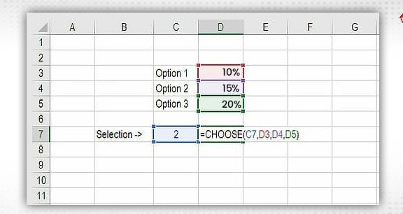
10. CHOOSE
The CHOOSE function is an excellent tool for scenario analysis in financial modelling, allowing users to select from multiple options and return a specific choice.
*janbasktraining.com
The formula is structured as =CHOOSE(index_num, value1, value2, value3, …), where index_num determines which value to return based on its position. For instance, if you have three projected values for income growth next year based on different assumptions, you can use the CHOOSE function to return the relevant amount, making it a valuable asset for decision-making in financial contexts.
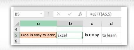
11. LEFT, RIGHT, MID
The LEFT(), RIGHT(), and MID() functions in Excel are essential for text manipulation, each serving a unique purpose.
- LEFT(): This function extracts a specified number of characters from the beginning of a text string. For example, if you have the text “Excel Functions” in cell A1 and use the formula =LEFT(A1, 5), it will return “Excel.”
- MID(): This function retrieves a substring from a text string, starting at a specified position for a specified length. For example, using =MID(A1, 7, 8) on “Excel Functions” would return “Functions,” starting with the 7th character and taking 8 characters in total.
- RIGHT(): This function extracts characters from the end of a text string. For instance, =RIGHT(A1, 8) applied to “Excel Functions” would yield “Functions” as well, pulling the last eight characters.
These text functions are not only useful for data analytics but also play a significant role in SQL and other data management tools. If you’re considering a career in this field, pursuing an online SQL certification could be beneficial.
*janbasktraining.com
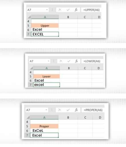
12. UPPER, LOWER, PROPER
The UPPER(), LOWER(), and PROPER() functions are valuable for formatting text strings in Excel.
- UPPER(): This function converts all letters in a text string to uppercase. For example, =UPPER(“Hello”) would return “HELLO.”
- LOWER(): Conversely, the LOWER() function transforms all letters in a text string to lowercase. For instance, =LOWER(“WORLD”) would return “world.”
- PROPER(): This function capitalises the first letter of each word in a text string while converting all other letters to lowercase. For example, =PROPER(“Hello World”) would return “Hello World.”
13. NOW()
The NOW() function is a straightforward way to obtain the current system date and time in Excel. This function updates every time the worksheet is edited or opened, providing real-time information. Since it does not require any arguments, simply entering =NOW() will return the current date and time, which can be formatted to display just the date or include the time as needed.

*janbasktraining.com
14. XNPV and XIRR
For analysts involved in investment banking, equity research, or any financial sector requiring cash flow analysis, the XNPV and XIRR functions are invaluable.
- XNPV: This function calculates the net present value (NPV) of an investment based on a specific discount rate and cash flows that occur at irregular intervals. The formula is structured as =XNPV(discount_rate, cash_flows, dates), making it a powerful tool for financial analysis.
- XIRR: This function determines the internal rate of return (IRR) for a series of cash flows occurring at irregular intervals. The formula is =XIRR(values, dates, [guess]), providing insights into the profitability of investments.
15. RANDBETWEEN
The RANDBETWEEN() function generates a random integer within a specified range. For example, using the formula =RANDBETWEEN(1, 100) will return a random number between 1 and 100. This function is useful for simulations and testing scenarios where random data points are required.
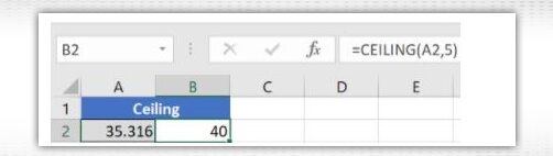
16. CEILING
The CEILING() function rounds a number up to the nearest specified multiple. For instance, if you use =CEILING(45.316, 5), it will round up to the nearest multiple of 5, resulting in 50. This function is particularly useful for financial calculations where rounding rules must be applied.
*janbasktraining.com
17. CONCATENATE
The CONCATENATE() function merges multiple text strings into a single string. The formula is structured as =CONCATENATE(text1, text2, [text3], …). For example, =CONCATENATE(“Hello “, “World”) would yield “Hello World”. This function can gather up to 30 values, making it a powerful tool for combining data.
18. LEN
The LEN() function returns the total number of characters in a text string, including spaces and special characters. The syntax is =LEN(text). For example, =LEN(“Excel”) would return 5, as it counts all the letters in the word.
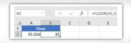
19. FLOOR
In contrast to the CEILING function, the FLOOR() function rounds a number down to the nearest specified multiple. For example, =FLOOR(45.316, 5) would result in 45, rounding down to the nearest multiple of 5.
*janbasktraining.com
20. REPLACE
The REPLACE() function allows you to substitute a portion of a text string with another string. The syntax is =REPLACE(old_text, start_num, num_chars, new_text). Here, start_num indicates the position in the text where the replacement begins, and num_chars specifies how many characters to replace. For instance, =REPLACE(“Hello World”, 7, 5, “Excel”) would change “World” to “Excel”, resulting in “Hello Excel”.
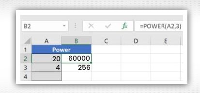
21. POWER
The POWER() function in Excel determines a number raised to a given exponent. The POWER() function is a quick way of doing exponentials. For example, you would enter =POWER(A2,3) to compute the value of the number in cell A2 (assume A2 is valued at 10) raised to the power of 3. This calculation results in 1000 (in this case, this is 10^3 = 100010^3 = 1000). Being proficient with the POWER function can make complex calculations easier in several disciplines, including data science. If you’re new to using this function and want to get better at it, you could enrol in a certification course for data science.
*janbasktraining.com
22. SMALL
The SMALL() function returns the nth smallest value from a set of numerical values so that users can retrieve the data values for specific criteria applied to the sorted order of values. The syntax for the function is =SMALL(array, k), where array is each of the cells with the data, and k is the order of the smallest value you want to return.
For example, if you had a given range indicating sales in a specific manner, =SMALL(A1:A10, 2) would return the second smallest value from that range. The SMALL() function can be used as a tool to analyse datasets while also reporting key performance metrics.
23. SUBSTITUTE
The SUBSTITUTE() function will replace instances of one substring with another substring in a text string.
The syntax for the function is =SUBSTITUTE(text, old_text, new_text, [instance_num]).
For example, assume cell A20 contains “I like apples.” To substitute “I like” with “She likes”, you would enter =SUBSTITUTE(A20, “I like”, “She likes”). As a result, “She likes apples” will be returned, quickly substituting part of a string without having to find and replace it manually.
24. QUARTILE
The QUARTILE() function takes a dataset and divides it into four equal portions so users can evaluate how data values are distributed.
The function is written as =QUARTILE(array, quart), where array contains the dataset and quart is the quartile being requested (0 is the minimum value, 1 is the first quarter of the dataset, 2 is the median, 3 is the last quarter of the dataset, 4 is the maximum value).
As an example, =QUARTILE(A1:A10, 1) will return the first quarter of the values of A1 through A10. This function can be useful when performing statistical evaluations and trying to understand the distribution of datasets.
25. OFFSET Combined with SUM
The OFFSET() function is used for dynamic references in Excel, which can be very powerful in working with SUM().
OFFSET() isn’t the most useful function alone, but with SUM, it can sum a variable range of Excel values. The formula would be in the following format: =SUM(Start Cell: OFFSET(Start Cell, 0, End Cell)).
This format will allow for some counting of values in an effective and dynamic range instead of editing them each time the dataset is updated.
26. IF AND
The IF() and AND() functions can both be used together to check multiple conditions in a dataset. This capability is quite helpful for classifying data following specific conditions.
For example, you could use the following formula to identify employees with salaries above $60,000 and employee IDs above 5: =IF(AND(E4>5, F4>60000), 1, 0). If both conditions are met, the formula will return 1; otherwise, the formula will return 0. This functionality assists in making reports and dynamic analyses based on user-defined conditions.
27. Pivot Tables
The IF() and AND() functions can both be used together to check multiple conditions in a dataset. This capability is quite helpful for classifying data following specific conditions.
For example, you could use the following formula to identify employees with salaries above $60,000 and employee IDs above 5: =IF(AND(E4>5, F4>60000), 1, 0). If both conditions are met, the formula will return 1; otherwise, the formula will return 0. This functionality assists in making reports and dynamic analyses based on user-defined conditions.
28. Pivot Table Slicers
Slicers enhance the usability of pivot tables by providing a visually appealing way to filter data. Instead of traditional drop-down menus, slicers present buttons that allow users to quickly hide or show specific data elements. By interacting with slicers, users can dynamically filter the data displayed in the pivot table, making it easier to focus on particular subsets of information. This intuitive feature simplifies data exploration and helps users gain insights more efficiently.
29. Macros
Macros in Excel are user-defined commands that automate repetitive tasks, allowing for streamlined processes and increased efficiency. By recording a series of actions, users can execute these commands automatically whenever needed. For example, you could create a macro to generate a custom table from your accounts receivable data, applying specific criteria such as date restrictions and formatting rules to highlight overdue payments in red. Understanding and utilising macros can significantly enhance productivity by reducing the time spent on manual tasks.
30. Flash Fill
Excel’s Flash Fill is a fantastic way to save time by automatically filling data as you develop a pattern. Flash Fill can be particularly helpful when needing to break full names into first and last names or bring names together from two different columns into just one! When you develop a pattern, Flash Fill will automatically populate the rest of the cells in the remaining column. Flash Fill is a reliable tool that will help you obtain better efficiency and accuracy in your data management tasks! It is a great feature to have in your Excel toolbox!
Pro Tips for Mastering Microsoft Excel
Congratulations on entering the world of Excel! You’ve gotten the basics down and learnt a few formulas, so let’s look at some professional tips to take your Excel game to a new level.
Save Smart
When working on your masterpieces in Excel, always consider backward compatibility. If you use functions only available in a newer version of Excel, be sure to save the file in the old 2003 format (*.xls) so that older versions will remain compatible with your brilliant work!
Name It Right
Using descriptive names is highly beneficial. Clearly label your columns and worksheets. The labelling will make your workbook more user-friendly, and it will also give outsiders an easy way to understand your data.
Keep It Simple
Complex equations can be overwhelming, so why not divide them into smaller, more manageable pieces? This will help simplify your calculations and make it easier to troubleshoot if things go wrong.
Use Predefined Functions
Rather than unnecessarily complicate things with complex formulas, use a function that Excel already has. That’s what they are there for! Using these functions will save you time and mistakes.
In the End
Excel is indeed an effective platform for analysing and reporting data. By this point, you have learnt the important Excel formula lists and functions that can make your projects simpler and quicker. Being proficient in Excel will increase your employment prospects, as 1 in 8 people use it worldwide. If you’re interested in some online IT courses to enhance your learning, see what we offer at Jaro Education!

Frequently Asked Questions

