
- jaro education
- 5, May 2024
- 10:00 am
Machine learning, a vital part of artificial intelligence, involves creating algorithms and statistical models to learn from data and make predictions. One such algorithm is linear regression, which falls under supervised machine learning. In supervised learning, algorithms learn from labeled datasets, mapping data points to optimized linear functions for prediction on new datasets.
To grasp linear regression fully, it’s essential to understand supervised machine learning. In this type of learning, algorithms learn from labeled data, where each data point has a known target value. Supervised learning includes two key types, classifications and regression.
Classification involves predicting the category or class of a dataset using independent input variables. This typically deals with categorical or discrete values, such as determining whether an image depicts a cat or a dog. Regression, on the other hand, focuses on forecasting continuous output variables based on independent input variables. For instance, it can predict house prices by considering various parameters such as house age, distance from the main road, location, and area.
From understanding simple and multiple linear regression to unveiling its significance, limitations, and practical use cases, you will get a comprehensive understanding of linear regression.
What is Linear Regression?
Table of Contents
Linear regression is a frequently utilized method for predictive analysis that clearly defines the relationship between continuous variables. It demonstrates the linear correlation between the independent variable (on the X-axis) and the dependent variable (on the Y-axis), thus the term linear regression. Simple linear regression is defined as having only one input variable (x). Multiple linear regression, on the other hand, is used when several input variables are involved. Essentially, the linear regression model provides a straight line with a predetermined slope that depicts the connection between variables.
Linear regression serves as a predictive instrument and also lays the groundwork for numerous sophisticated models. Some of the methods, such as regularization and support vector machines, are influenced by linear regression. Moreover, linear regression plays a pivotal role in assumption testing, allowing researchers to verify crucial assumptions regarding the dataset.
Type of Linear Regression
As discussed above there are two main types of Linear Regression
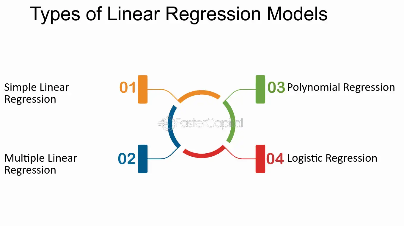
Simple Linear Regression
Simple Linear Regression is a fundamental statistical method used to understand the relationship between two continuous variables. In this model, we have a predictor variable (X) and a response variable (Y), and we assume that there is a linear relationship between them. The aim is to find a straight line that best fits the data points, allowing us to make predictions based on new values of the predictor variable.

Here:
- Y represents the response variable (the variable we want to predict).
- X represents the predictor variable (the variable we use to make predictions).
- Β0 is the intercept, which represents the value of Y when X is 0.
- Β1 is the slope, it shows the change in Y for a one-unit change in X.
- ε represents the error term
Here Simple Linear Regression is used to determine the values of β0 and β1 that minimize the sum of squared variances between observed Y values and those predicted by the regression line. Once the regression coefficients (β0 and β1) are calculated, we can utilize the regression equation to forecast Y values for new X values. This involves substituting the new X values into the equation to derive the predicted Y values.
Multiple Linear Regression
Multiple linear regression extends this concept to analyze the relationship between two or more independent and dependent variables. The equation for multiple linear regression is
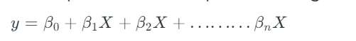
Here in this equation,
- Y is the dependent variable
- X1, X2, …, Xp are the independent variables
- β0 is the intercept
- β1, β2, …, βn are the slopes
The objective of multiple linear regression remains the same: to find the coefficients that minimize the difference between observed and predicted values. Furthermore, multiple linear regression allows for more complex modeling of relationships involving multiple factors.
The algorithm aims to find the best Fit Line equation for predicting values using independent variables.
In regression analysis, we use a dataset with X and Y values to train a function. This function then helps predict Y values when given an unknown X input. In regression, we’re essentially figuring out the value of Y, so we need a function that can predict continuous Y values based on independent features X.
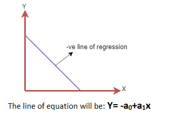
Linear Regression Line
A regression line illustrates the connection between dependent and independent variables and is characterized by its linearity. This line depicts two main types of relationships:
Positive Linear Relationship: This type of relationship occurs when the dependent variable increases along the Y-axis while the independent variable increases along the X-axis. It is referred to as a positive linear relationship.
Cost Function
The cost function is essential for determining the optimal values of a0 And a1 that yield the most suitable line of best fit for the given data points. This function serves to optimize the regression coefficients or weights and assesses the performance of a linear regression model. Its primary purpose is to evaluate the accuracy of the mapping function, also referred to as the Hypothesis function, which maps the input variable to the output variable.
In the context of Linear Regression, the Mean Squared Error (MSE) is commonly employed as the cost function. MSE represents the average of the squared errors between the predicted values and the actual values.
The MSE for a simple linear equation y=mx+b can be calculated as:
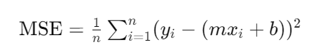
Where,
N=Total number of observations
Yi = Actual value
(mxi+b0)= Predicted value.
Gradient Descendent
Training a linear regression model involves utilizing the gradient descent optimization algorithm. This iterative approach adjusts the model’s parameters to minimize the mean squared error (MSE) observed on the training dataset. By updating the values of θ1 and θ2, the model aims to reduce the Cost function, thereby minimizing the root mean squared error (RMSE) and achieving the optimal fit for the data. Gradient Descent is employed to iteratively refine these parameter values, beginning with random initialization and progressively moving towards minimizing the overall cost.
Essentially, gradients represent derivatives that indicate how changes in inputs affect the outputs of a function.
Model Performance
The evaluation of model performance relies on assessing how well the regression line aligns with the observed data points. This process, known as optimization, involves selecting the most suitable model from a range of options. One method for achieving optimization is through the application of the R-squared metric:
- R-squared, a statistical measure, evaluates the goodness of fit of a model.
- It quantifies the strength of the relationship between independent and dependent variables, expressed on a scale from 0 to 100%.
- A high R-squared value indicates a minimal disparity between predicted and actual values, signifying a well-fitting model.
- Additionally referred to as the coefficient of determination, in the context of multiple regression analysis, it is termed the coefficient of multiple determination.
- The R-squared value can be computed using the following formula:

Assumptions of Linear Regression
Linear regression relies on several key assumptions to ensure the accuracy and reliability of the model. These considerations help optimize the performance of the linear regression model when working with a given dataset.
- Linear Relationship: Linear regression presupposes a direct linear relationship between the independent variables (features) and the dependent variable (target). This suggests that as one variable changes, the other changes proportionally.
- Multicollinearity: Multicollinearity denotes the correlation between independent variables. High multicollinearity may obscure the genuine relationship between predictors and the target variable. Hence, linear regression expects minimal or no multicollinearity among the features.
- Homoscedasticity: Homoscedasticity signifies that the variance of the errors remains consistent across all values of the independent variables. Essentially, it denotes that the dispersion of data points around the regression line remains constant throughout the range of predictors.
- Normal Distribution of Errors: Linear regression presupposes that the errors (residuals) adhere to a normal distribution. This ensures that the statistical properties of the model, such as confidence intervals, remain precise. A common approach to validate this assumption is through a q-q plot, which should exhibit a straight line if the errors are normally distributed.
- No Autocorrelation: Autocorrelation arises when there is a correlation between the residuals themselves. Linear regression assumes the absence of such correlation, as it can yield inaccurate estimates of the model coefficients. Autocorrelation typically emerges when there is a pattern or dependency in the residual errors.
- Independence of Observations: Linear regression assumes that the observations or data points are independent of each other. Put simply, the value of one observation does not impact the value of another observation. This assumption ensures that each data point furnishes unique information to the model and averts biases in the estimation process.
Multicollinearity
Multicollinearity is a statistical occurrence wherein two or more independent variables within a multiple regression model exhibit high correlation, thereby complicating the assessment of each variable’s individual impact on the dependent variable.
Identification of Multicollinearity involves employing two methods:
- Correlation Matrix: This approach involves scrutinizing the correlation matrix among the independent variables. Elevated correlations (near 1 or -1) signify potential multicollinearity.
- VIF (Variance Inflation Factor): VIF serves as a metric that measures the extent to which the variance of an estimated regression coefficient increases due to correlated predictors. A VIF exceeding 10 typically indicates multicollinearity.
Pros and Cons of the Linear Regression Method
Linear regression is a popular statistical approach in machine learning for predicting a dependent variable based on one or more independent variables. Let’s divide it down into positives and cons.
Advantages:
Simplicity: It’s easy to implement and understand the output coefficients.
Interpretability: The model provides clear coefficients, helping us understand each independent variable’s impact.
Quantification of Relationships: It lets us quantitatively grasp how variables relate to each other.
Less Complexity: When the relationship between variables is linear, it’s the simplest choice compared to other algorithms.
Diagnostic Tools: Offers tools to assess model quality and spot potential issues.
Disadvantages:
Assumption of Linearity: It assumes variables have a linear relationship, which may not always be true.
Effect of Outliers: Outliers can greatly affect the regression, potentially skewing results.
Oversimplification: It might overly simplify real-world problems by assuming linear relationships among variables.
Risk of Overfitting: Though techniques like regularization and cross-validation can help, there’s still a risk of overfitting.
Independence of Observations: Assumes all observations are independent, which might not be true in clustered data.
Conclusion
Linear regression is a profound machine learning method. It’s often used because it’s simple, easy to understand, and works well. It helps us understand how different things are related and make predictions in many different areas.
However, it’s important to know its limits. It assumes that relationships are straight lines and can struggle when variables are closely connected. By being careful about these issues, though, linear regression can still be really useful for exploring data and making predictions. You can learn machine learning concepts in depth from Online Master of Science (Data Science) – Symbiosis School for Online and Digital Learning (SSODL), designed to give a thorough foundation in data science and machine learning, including their lifecycle, statistical underpinnings, technological tools, and practical uses. Crafted by seasoned experts of Symbiosis’s renowned B-School, the curriculum promises top-tier education that is equivalent to pursuing an offline MBA degree.
Trending Blogs